Overview
Stochastic constructive design optimization refers to a class of algorithms that build complex structures iteratively by adding components (e.g. vessel segments) in accordance to some optimization rules and some additional constraints. In vascular modeling, the prototypical example is Constrained Constructive Optimization (CCO)-an algorithm introduced by Schreiner & Buxbaum (1993) for generating arterial trees. CCO and its related algorithms have become gold-standard techniques for synthesizing plausible vascular networks in silico Karch et al. (1999). Recent open implementations (e.g., OpenCCO) and adaptive variants (Sci Rep 2021) have continued to extend the capabilities of this group of algorithms. These algorithms strive to mimic physiological design principles including balancing metabolic supply and pumping energy (Murray's Law) so that synthetic vessels closely resemble the geometry and hemodynamics of native networks. The construction is stochastic because each new vessel insertion involves a random or pseudo-random sampling of points within the build space followed by appropriate constraints and an optimization step to integrate that vessel at a bifurcation point. Over many iterations, this yields a branching network that "grows" throughout the build space. Often, these networks exhibit fractal-like properties reminiscent of native blood vessels. These algorithms are powerful in biomedical research, allowing investigators to simulate microvascular architectures for different organs, conditions, or species where imaging data is sparse.
Core ideas
- Constructive growth: Start from a seed; add elements (nodes, segments, primitives) one at a time.
- Feasibility at every step: Enforce hard constraints (e.g., geometry, non-overlap, boundary conditions) during growth.
- Local optimization: After each addition, adjust a small neighborhood (topology, positions, radii, weights) to improve an objective.
- Greedy–stochastic blend: Explore candidates stochastically; accept using greedy or tempered criteria.
- Anytime property: You can stop early and still have a valid, usable design.
One growth cycle
Local Bifurcation Optimization
For a fixed target \(X\), choose the best feasible proposal \(p\) by minimizing an objective \(J\):
Local refinement (bifurcation position \(b\) and radii \(r\)) over a neighborhood \(\mathcal{N}\):
In practice, \(J\) is a penalized composite that combines hemodynamic power \(\sum_i R_i Q_i^2\) with geometric costs (e.g., total volume/length and smoothness/turning penalties); the flows \(Q_i\) are obtained from a fast 0D (Poiseuille) solve for each candidate. Hard constraints (domain inclusion, segment–segment clearance, degree limits) are enforced as feasibility filters—candidates failing a cheap pre-check are discarded—or equivalently via an indicator \(\iota_{\mathcal{F}}(p)\in\{0,\infty\}\) added to \(J\). Soft constraints (angle/taper bounds, min radius, curvature) are added as penalties, e.g., \(\mu\sum_i \big[\!g_i(p)\big]_+^2+\nu\sum_j h_j(p)^2\); the Murray relation \(r_0^{\,n}=r_1^{\,n}+r_2^{\,n}\) (typically \(n\approx 3\)) is enforced either exactly (equality) or via a strong penalty while optimizing \(b\) and \(r\). The local search is low-dimensional in practice: move \(b\) along a bounded segment/plane and update radii from the flow split, using a short line search or trust-region step; the accepted proposal is the feasible candidate with the smallest penalized \(J\), otherwise the routine resamples/relaxes (anneals) if no candidate passes.
Typical CCO pipeline
- Initialize a feasible seed (root node, inlet, or minimal skeleton).
- Sample a target (demand point, region of interest, or heuristic focus).
- Propose connections from the existing structure to the target (multiple candidates).
- Project & sanitize into valid space (snap to domain, avoid collisions/violations).
- Local optimize the neighborhood (positions, radii/weights, minor topology tweaks).
- Evaluate constraints and score the objective (with penalties for soft rules).
- Select the best feasible candidate; commit to the structure.
- Repeat until coverage/quality targets are met or a budget is exhausted.
Objectives & constraints
| Type | Examples | Notes |
|---|---|---|
| Objective | Minimize cost/length, imbalance, pressure drop, or a weighted composite | Often additive across elements; may include regularizers. |
| Hard constraints | Geometric validity, non-intersection, boundary inclusion, degree limits | Must hold at every step; violated candidates are rejected. |
| Soft constraints | Preferred angles, tapering rules, smoothness | Typically encoded as penalties in the objective. |
Data structures that help
- Spatial index (k-d tree, BVH) for nearest-neighbor queries and fast collision checks.
- Adjacency graph (nodes/edges) to update local neighborhoods efficiently.
- Constraint cache to memoize expensive checks (e.g., local clearance or regional quotas).
- Candidate pool with ranked proposals and provenance for reproducibility.
Deep-dive: how this maps to svVascularize
The svVascularize API follows the CCO pattern and exposes hooks to control sampling, constraints, and local refinement:
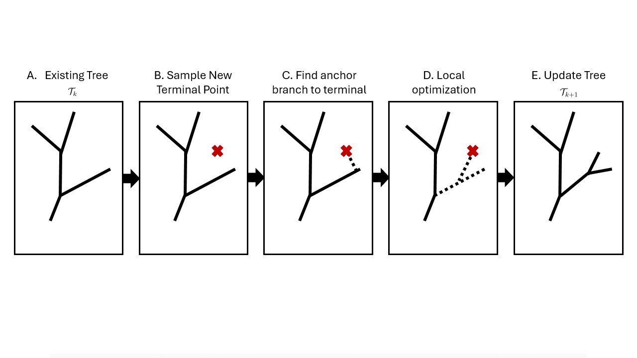
- Seed/init: create a root vessel and initial terminals inside the domain (mesh/voxel/signed-distance). (CCO: minimal feasible \(S_0\)).
- Target sampling: draw a terminal location \(X\) (uniform, blue-noise, or demand-weighted) to improve coverage.
- Candidate proposals: choose anchors (nearby segments/terminals) and propose a dashed path to \(X\); project into the domain and sanitize (clearance, no self-intersection).
- Local optimization: refine bifurcation position and daughter radii under Poiseuille/Murray constraints to minimize \(J\).
- Feasibility check: accept only if hard constraints pass; otherwise resample or relax.
- Commit & update: add solid segments to obtain \(S_{k+1}\), update flows/pressures and spatial indices.
Typical objective and constraints
| Type | Examples | Notes |
|---|---|---|
| Objective | \(J = \alpha\,\text{Power} + \beta\,\text{Volume} + \gamma\,\text{Smoothness}\) | Weights \(\alpha,\beta,\gamma\) tune energy vs material vs geometry. |
| Hard constraints | Domain inclusion, non-intersection, degree limits, inlet/outlet boundary rules | Reject on failure (no penalties). |
| Soft constraints | Preferred angles, taper, min/max radius | Encode as penalties within \(J\). |
Pseudocode for CCO processes
The loop below mirrors the implementation pattern.
def cco(seed, domain, params):
    T = initialize_structure(seed, domain, params)       # T_{0}
    while not done(T, params):
        X = sample_target(domain, T, params)             # fixed target for this iteration
        candidates = []
        for a in select_anchors(T, X, params):
            p = propose(a, X, params)                    # dashed proposal
            p = project_and_sanitize(p, domain, T)       # enforce geometry/bounds
            (b_star, r_star) = local_optimize(p, T, params)
            if hard_constraints_ok(T, p, b_star, r_star, domain):
                score = objective(T, p, b_star, r_star, params)  # J(...)
                candidates.append((score, (p, b_star, r_star)))
        if not candidates:
            handle_stall(T, X, params)                   # resample/relax; keep feasibility
            continue
        _, best = min(candidates, key=lambda t: t[0])     # argmin over feasible
        T = commit(T, *best)                              # accept → T_{k+1}
    return T
Related stochastic generators
- Simulated-annealing vascular optimization (SALVO): global re-wiring via Metropolis updates; see Sci Rep 2021 and arXiv 2020.
- Growth-based optimization (GBO): tissue-demand-guided constructive growth; see Kim et al., 2023 and MRI perfusion validation in Rundfeldt et al., 2024.
- L-systems / fractal generators: procedural branching with Murray-style rules; e.g. Ritraksa et al., 2021.
- More global formulations: continuous/integer programs or constructive-global hybrids; e.g. WUSTL technical report.