svVascularize

Quickstart tutorial

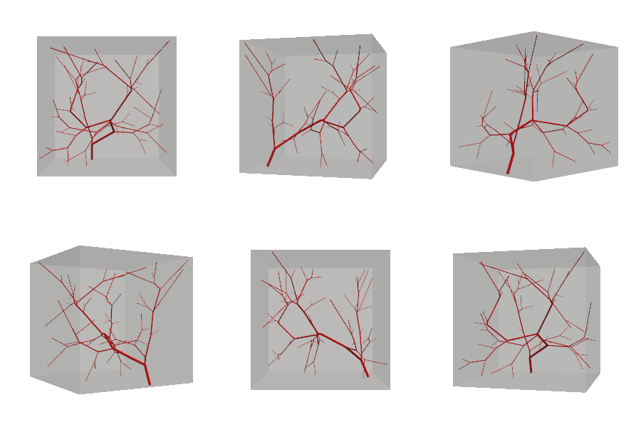
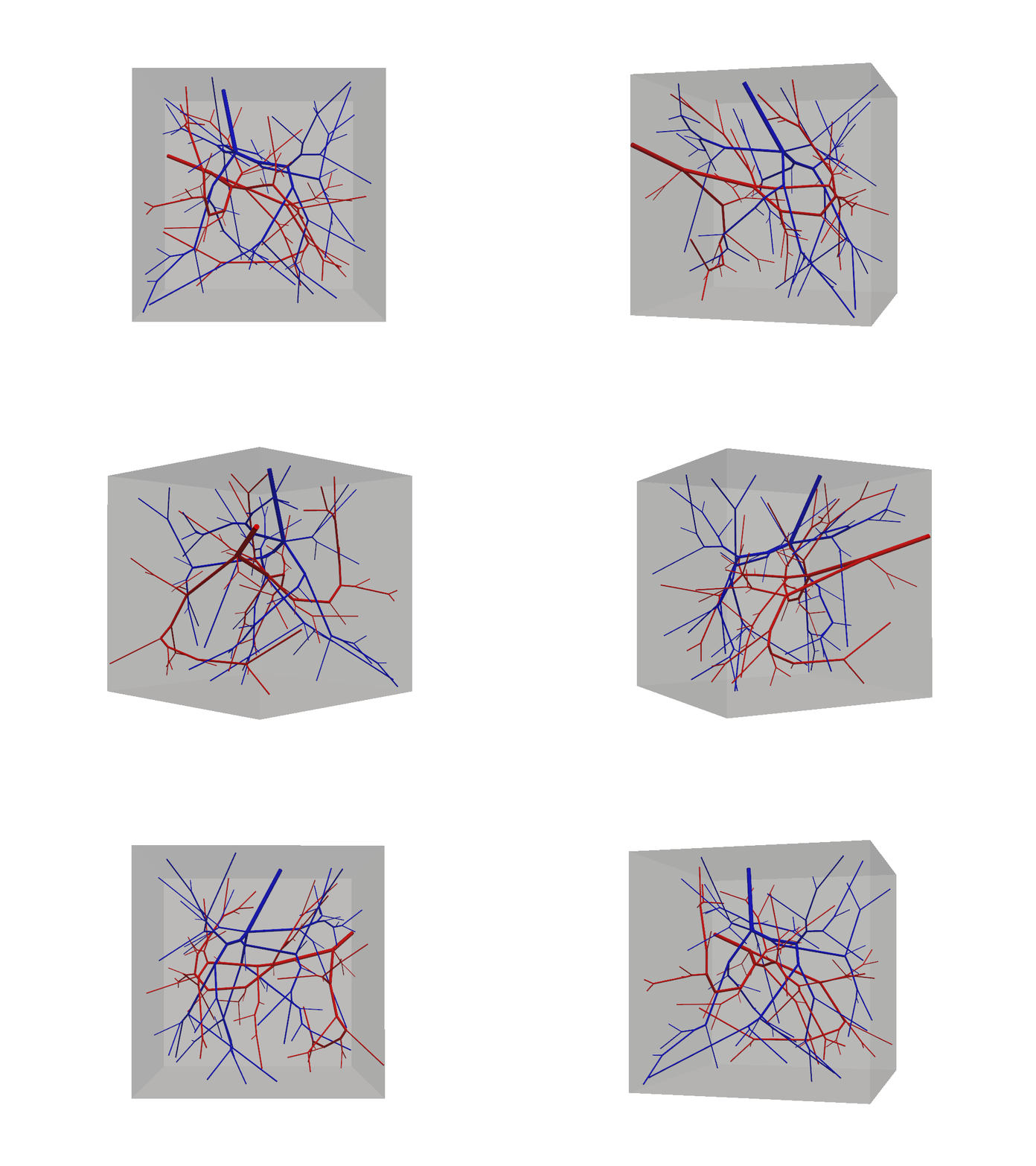
This guide shows how to grow a small synthetic vascular objects and export 0‑D simulation files for a simple convex shape. For this example we will forgo including other build parameters such as starting points and additional hemodynamic constraints in order to focus on only the essential API for minimally viable vascular objects. Here we create a simple domain, grow a vascular tree and forest, visualising them in an interactive viewer, and export 0‑D hemodynamic simulation files for further analysis using svzerodsolver .

Generate and visualise a tree

import pyvista as pv
from svv.domain.domain import Domain
from svv.tree.tree import Tree

# Creating the Tissue Domain
cube = Domain(pv.Cube())
cube.create()
cube.solve()
cube.build()

# Creating the Vascular Tree Object
t = Tree()
t.set_domain(cube)
t.set_root()
t.n_add(50)

# Visualizing the Tree and Domain
t.show(plot_domain=True)

Export 0‑D simulation files

from svv.simulation.fluid.rom.zero_d.zerod_tree import export_0d_simulation

export_0d_simulation(t, outdir="my_tree_0d")

This writes a 0-D solver input file, solver_0d.in, and geometric file, geom.csv, in the folder my_tree_0d/. The input file should contain all necessary parameters and inflow conditions to run the simulation. By default, 0-D simulations exported via this routine will simulate steady state flow through the vascular trees. Time-varying flows can be considered if additional arguments are applied to the export_0d_simulation function. Run the solver with svZeroDSolver.

Generate and visualise a forest

Unlike tree, forest objects are composed by connecting synthetic vascular trees to form fluid circuits with a desired number of inlets and outlets. These are especially useful for fabrication and fluid routing problems in which control over the start/end points are critical.

import pyvista as pv
from svv.domain.domain import Domain
from svv.forest.forest import Forest

# Creating the Tissue Domain
cube = Domain(pv.Cube())
cube.create()
cube.solve()
cube.build()

# Creating the Vascular Forest Object
f = Forest()
f.set_domain(cube)
f.set_roots()
f.add(50)

# Visualizing the Forest and Domain
f.show(plot_domain=True)

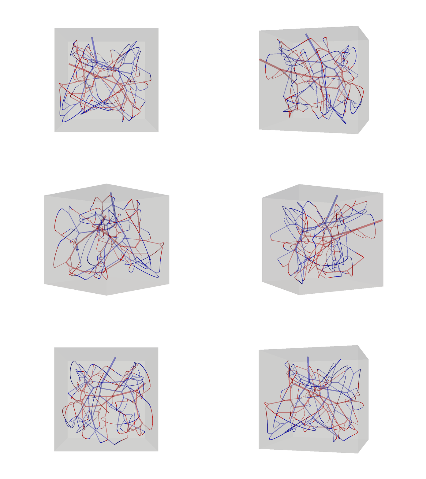
At this step our vascular forest object remains unconnected and should contain two non-intersecting trees. Because we have not specified any special build parameters, these trees adhere to the same default fluid constrains and are allowed to grow homogeneously within the tissue domain. Connections among multiple trees is accomplished via the forest.connect() method which automatically sets up a two-step optimization problem to form connections among sets of tree terminals.

# Form connections
f.connect()

# Visualize the Connected Forest Object
f.connections.tree_connections[0].show().show()

Export 0-D simulation files

Because a forest object may contain multiple fluid networks, it is important to specify which network a user wants to export for simulation as well as the inlet boundaries. These are the second and thrid positional arguments of the simulation exporting function, respectively.

from svv.simulation.fluid.rom.zero_d.zerod_forest import export_0d_simulation

export_0d_simulation(f, 0, [0], outdir="my_forest_0d")       

Similar to exporting the tree object for simulation, this function will write out a 0-D solver input file solver_0d.in as well as a geometric file, geom.csv for casting solutions back onto the 3D geometry for visualization. The inlet boundary conditions will be applied to the root vessel of the first tree since we specified this in the third argument of our function above. By default, this will be a steady flow simulation with a simple resistance outflow boundary condition. Solutions to the 0-D problem can be obtained using the same svzerodsolver workflow.